ArangoDB v3.11 reached End of Life (EOL) and is no longer supported.
This documentation is outdated. Please see the most recent stable version.
Data Loader Example
Follow this complete working example to see how easy it is to transform existing data into a graph and get insights from the connected entities
To transform your data into a graph, you need to have CSV files with entities representing the nodes and a corresponding CSV file representing the edges.
This example uses a sample data set of two files, airports.csv, and flights.csv.
These files are used to create a graph showing flights arriving at and departing
from various cities.
You can download the files from GitHub .
The airports.csv contains rows of airport entries, which are the future nodes
in your graph. The flights.csv contains rows of flight entries, which are the
future edges connecting the nodes.
The whole process can be broken down into these steps:
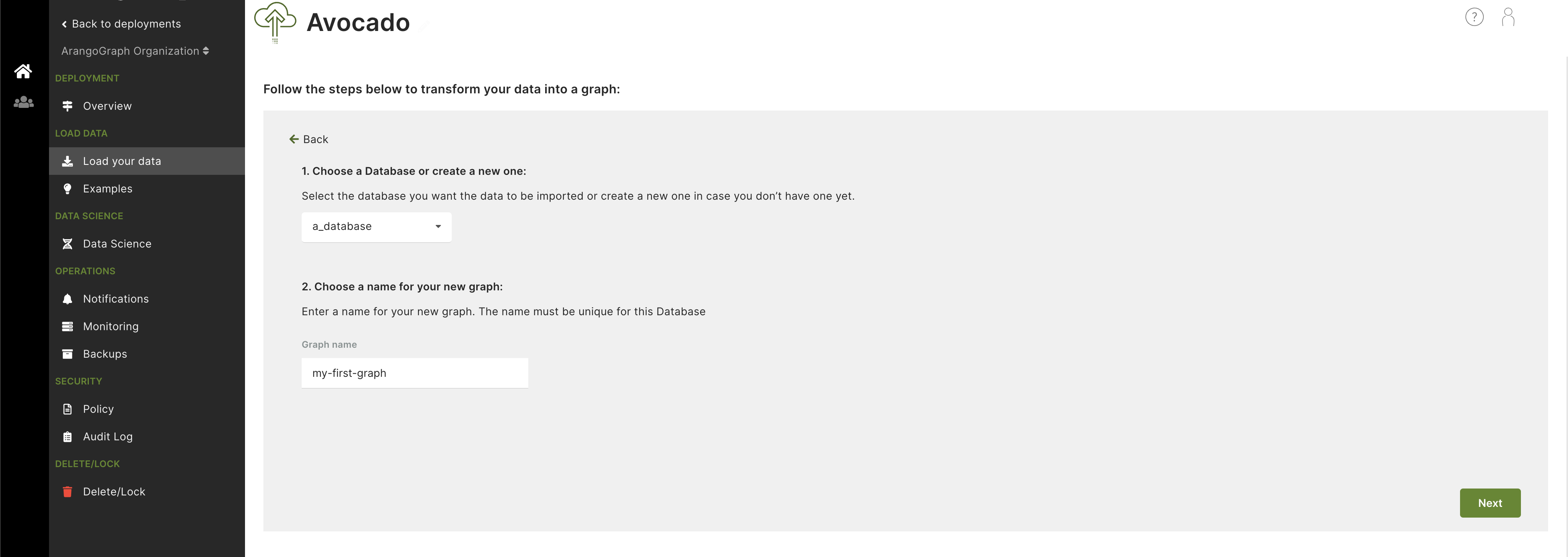
- Database and graph setup: Begin by choosing an existing database or create a new one and enter a name for your new graph.
- Add files: Upload the CSV files to the Data Loader web interface. You can simply drag and drop them or upload them through the file browser window.
- Design graph: Design your graph schema by adding nodes and edges and map data from the uploaded files to them. This allows creating the corresponding documents and collections for your graph.
- Import data: Import the data and start using your newly created EnterpriseGraph and its corresponding collections.
Step 1: Create a database and choose the graph name
Start by creating a new database and adding a name for your graph.
Step 2: Add files
Upload your CSV files to the Data Loader web interface. You can drag and drop them or upload them via a file browser window.
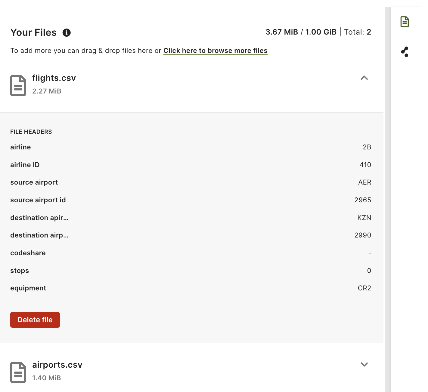
See also Add files into Data Loader.
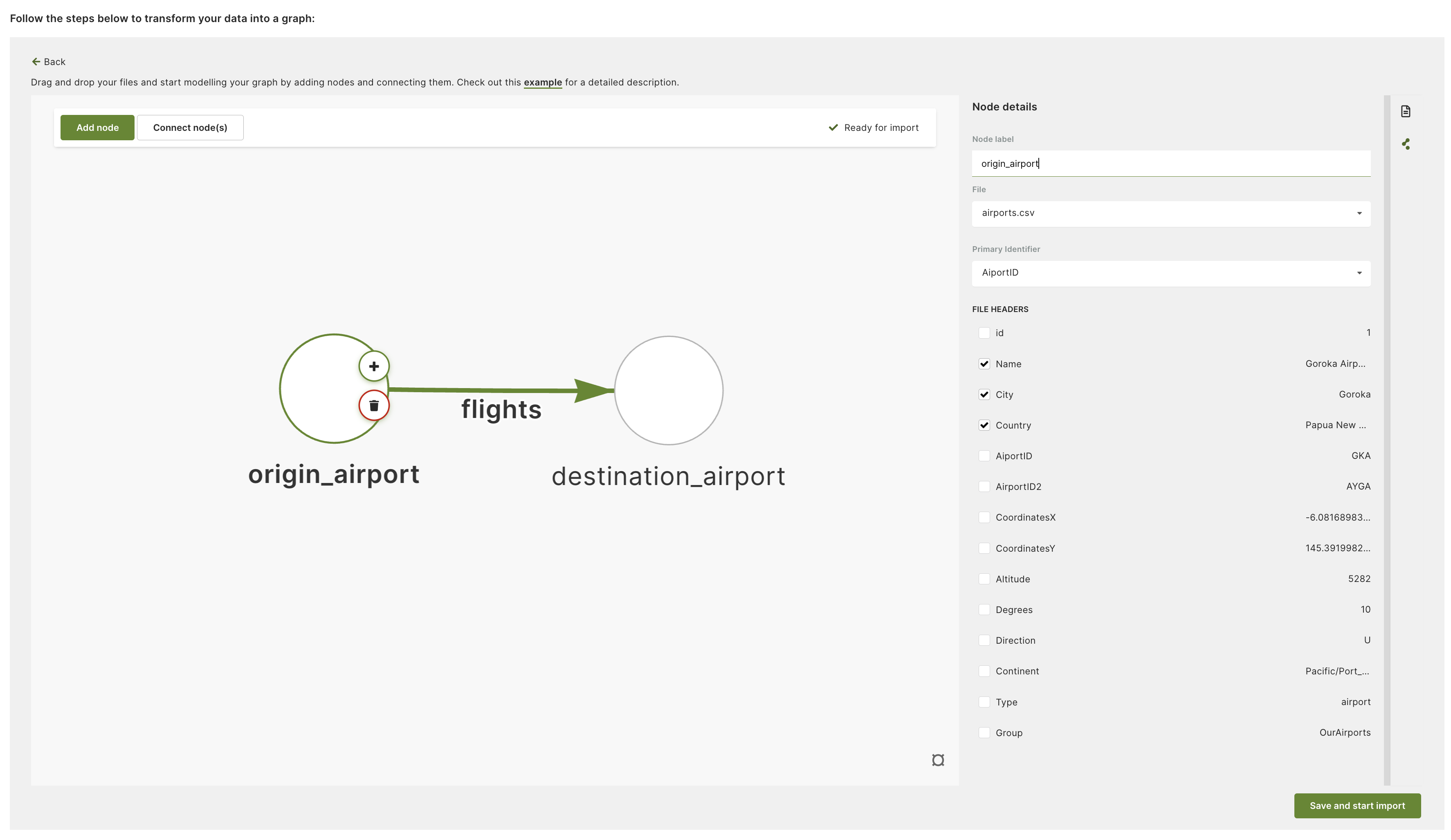
Step 3: Design graph schema
Once the files are added, you can start designing the graph schema. This example uses a simple graph consisting of:
- Two nodes (
origin_airportanddestination_airport) - One directed edge going from the origin airport to the destination one representing a flight
Click Add node to create the nodes and connect them with edges.
Next, for each of the nodes and edges, you need to create a mapping to the corresponding file and headers.
For nodes, the Node label is going to be a node collection name and the
Primary identifier will be used to populate the _key attribute of documents.
You can also select any additional headers to be included as document attributes.
In this example, two node collections have been created (origin_airport and
destination_airport) and AirportID header is used to create the _key
attribute for documents in both node collections. The header preview makes it
easy to select the headers you want to use.
For edges, the Edge label is going to be an edge collection name. Then, you
need to specify how edges will connect nodes. You can do this by selecting the
from and to nodes to give a direction to the edge.
In this example, the source airport header has been selected as a source and
the destination airport header as a target for the edge.
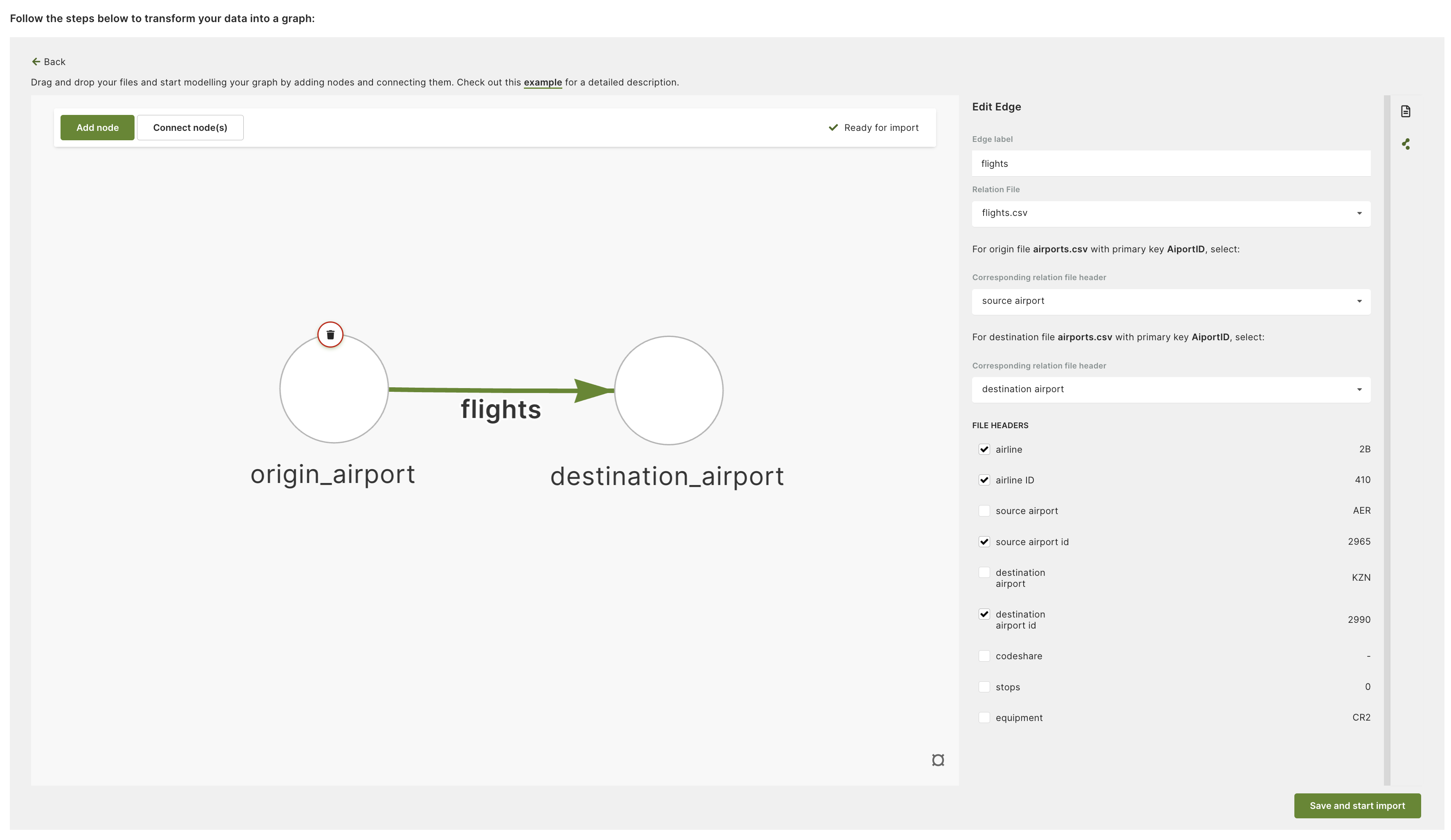
Note that the values of the source and target for the edge correspond to the
Primary identifier (_key attribute) of the nodes. In this case, it is the
airport code (i.e. GKA) used as the _key in the node documents and in the source
and destination headers to configure the edges.
See also Design your graph in the Data Loader.
Step 4: Import and see the resulting graph
After all the mapping is done, all you need to do is click Save and start import. The report provides an overview of the files processed and the documents created, as well as a link to your new graph. See also Start import.
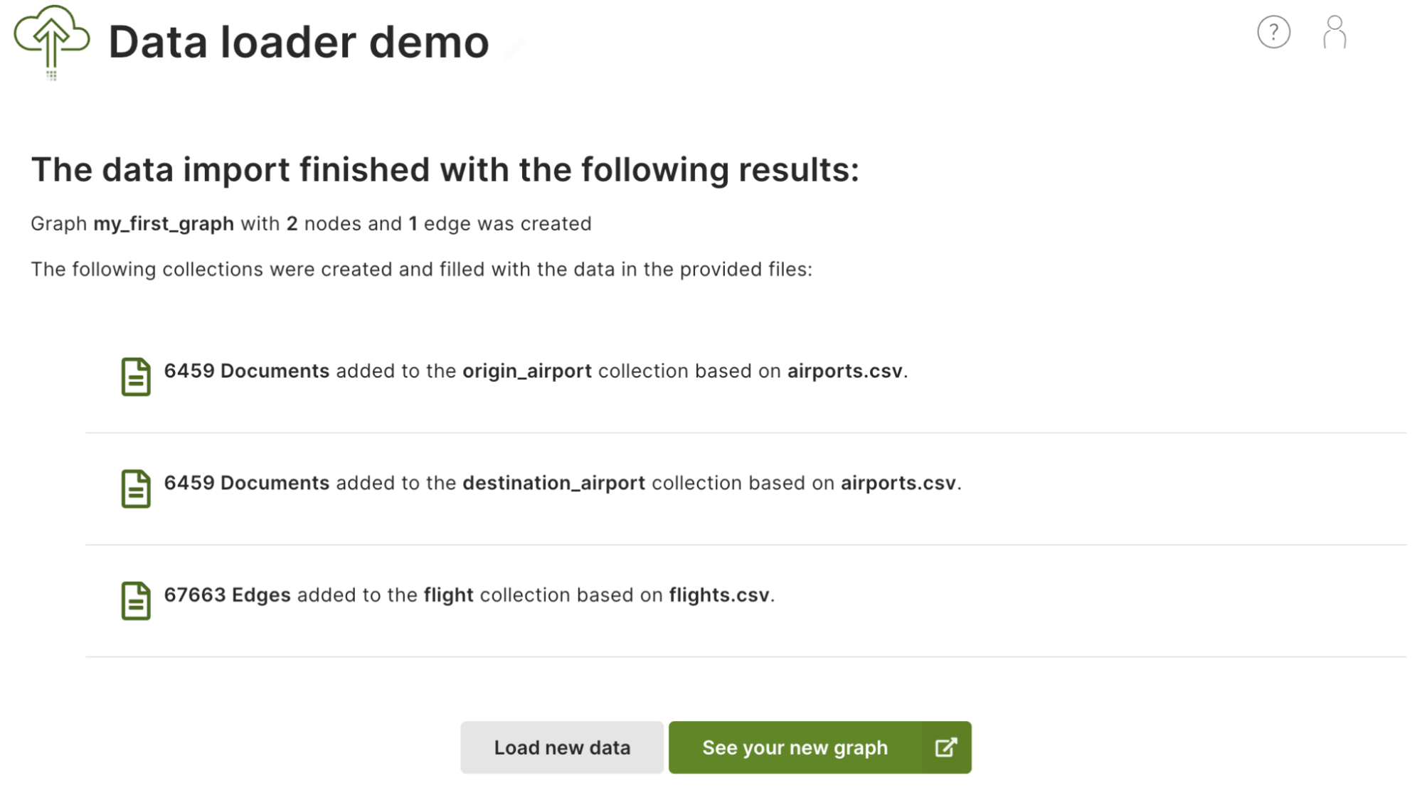
Finally, click See your new graph to open the ArangoDB web interface and explore your new collections and graph.
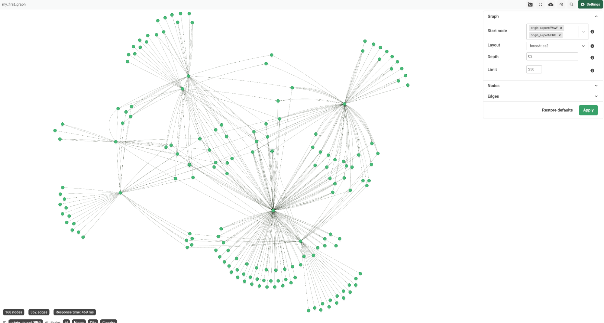
Happy graphing!